
This is a guest post by Keighley Rockcliffe.
Coronal Mass Ejections and the Skylab Mission
On May 14th, 1973, the US’s first space station, dubbed Skylab, was launched into low-Earth orbit on the last Saturn V rocket launch. Onboard Skylab was a workshop meant for the crew to perform experiments. These experiments covered research in biomedical science, solar and space physics, geology, material science and some student proposed studies. The habitability of the station itself was an experiment.

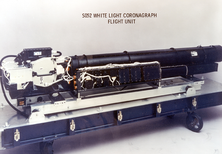
Skylab had its own solar observatory, the Apollo Telescope Mount, that included X-ray telescopes, UV measurement instruments, two Hydrogen-alpha telescopes, and a white light coronagraph. A coronagraph allows the faint outer atmosphere of the Sun to be observed by blocking the much brighter direct light from the solar disk. The High Altitude Observatory designed the coronagraph for Skylab, using an occulting disk to block light from the Sun’s disk and allow observation of the corona.
A star’s corona is a multi-component portion of the star’s outer atmosphere. Despite being farther away from the solar surface, the Sun’s corona is actually hotter than its surface by about 1000 times. The reason for this huge temperature discrepancy has been an active research topic since its discovery in the 1930’s and will be investigated by the recently launched Parker Solar Probe. The different parts of the corona are composed of light from different sources: Thomson scattered by electrons (K corona), scattered by dust (F corona), emission from ionized atoms (E corona), and some emission from the same dust contributing the F corona (T corona). The coronagraph within Skylab’s observatory allowed observation of the K corona, which makes up the brightest parts of the corona.
Some interesting and powerful events are visible within the corona, primarily involving the ejection of solar plasma and magnetic disturbances into the heliosphere. They are called coronal mass ejections (CMEs), traveling at speeds ranging from 100 to 3000 km/s and carrying around 10¹² kg of solar plasma (approximately the mass of Mount Everest). These eruptions can and do hit the Earth’s geospace, which can cause geomagnetic storms as well as barrage satellites and spacecraft with energetic particles. This motivates our current and past study of CMEs, solar flares, and the behavior of the corona.
For a nine-month period between 1973 and 1974, Skylab’s coronagraph took images of the Sun’s corona. Those images were originally on film, and the initial analysis was done using that medium. Recently the film frames were digitized, so in the last few months, I was tasked with using these images to create a catalog of the observed coronal mass ejections and their properties (location, projected speed, width). In order to look for these events, GIFs were made for each day of the mission containing all of the images taken that day. A few things needed to be altered about an image before creating a GIF.
Even with the help of the occulting disk, the coronagraph captured a lot of light which made it difficult to see events occur and propagate. A way to bypass this would be to manually mask the bright values closest to the Sun’s disk, which would allow the image scale to show more structure. For this, I used Python and the SunPy package. The information contained within each image header contains enough metadata to create a SunPy map. This is a spatially aware 2D array containing the image data along with metadata information and plot settings. Creating a map for each image file allowed the use of SunPy’s functions to manipulate maps. To solve the brightness problem, I used Numpy’s ‘meshgrid’ function to create a grid of pixels the size and shape of the image. SunPy’s map method ‘pixel_to_world’ then converts those pixels to solar coordinates (in this case, helioprojective Cartesian). From there, an array can be defined to represent the distance values of each pixel from the Sun’s center. Numpy’s function ‘masked_less_equal’ was then utilized to automatically mask the values of pixels within two solar radii of the Sun’s center. This allowed the dimmer parts of the corona to be visible.
The images were also misaligned due to the rotation of the instrument. The angle of Solar North (the Sun’s North pole) to the y axis of the image was recorded in each image’s header. SunPy’s ‘rotate’ method for the generic map automatically returned a new rotated map with the correct alignment. Importantly, all the SunPy map methods automatically update the spatial awareness of the map with no requirement on the user to perform the necessary coordinate transformations explicitly.
After all of those corrections were made to each image, a GIF per day was made over the course of the mission, using the Python library imageio. The imageio.imread() function can take a filename input and read that image in a specified format (PNG, EPS, JPEG, etc). Imageio.get_writer() can write the images read by imageio.imread() to a file of GIF format. In order to conserve space on my computer, I decided to loop through all of the data files associated with a day’s worth of images and create temporary PNG files of the corrected images which were then read by imageio and written into a GIF. A sample GIF is shown below that encompasses the images taken on August 10th, 1973. As you can see, a large coronal mass ejection occurs off of the Sun’s West limb. There are small shifts in the GIF (especially apparent when watching the axes) due to errors concerning some of the images’ metadata that have yet to be resolved.
With this processing, these unique historical data are now in a form that can be used to study properties of CMEs for a time when there were very few other observations of CMEs. This will enable us to better understand how the properties of CMEs depend on the solar cycle and will give us valuable insight into solar activity at a time when observations such as these were much rarer.